RESEARCH ARTICLE · DYNAMICAL SYSTEMS
Sharp Shadowability Bounds for Normal Hyperbolic Linear Operators
School of Mathematical Sciences, Beihang University
Beijing 100191, China
Abstract
Let \(A\) be an invertible normal hyperbolic operator on a complex Hilbert space \(H\). We obtain an exact spectral formula for the optimal uniform shadowability constant \(\operatorname{Shad}(A)\), sharpening the general additive Green-operator estimates to a Euclidean combination of the stable and unstable spectral contributions. If both spectral components are nonempty, set \[\alpha(A) = 1-\max\{|\lambda|:\lambda\in\sigma(A),\ |\lambda|<1\},\] and \[\beta(A) = \min\{|\lambda|:\lambda\in\sigma(A),\ |\lambda|>1\}-1.\] We prove the exact formula \[\operatorname{Shad}(A) = \left(\alpha(A)^{-2}+\beta(A)^{-2}\right)^{1/2},\] with the corresponding one-sided formulas when only one spectral component is present.
We further relate this exact constant to the robustness of hyperbolicity. Let \(r_{\mathrm{hyp}}(A)\) denote the operator-norm distance from \(A\) to the loss of hyperbolicity. We obtain the sharp universal ratio \[1\le r_{\mathrm{hyp}}(A)\operatorname{Shad}(A)\le\sqrt{2}.\] Both constants are optimal. In the mixed case, \[r_{\mathrm{hyp}}(A)\operatorname{Shad}(A) = \left[ 1+ \left( \frac{\min\{\alpha(A),\beta(A)\}} {\max\{\alpha(A),\beta(A)\}} \right)^2 \right]^{1/2}.\] Thus the normalized shadowability constant is determined exactly by the relative balance of the stable and unstable spectral gaps.
1. Introduction
The shadowing property is a fundamental notion in dynamical systems that describes whether approximate trajectories can be uniformly traced by exact trajectories. In the setting of linear dynamics, shadowing is closely related to spectral hyperbolicity, although the relationship becomes substantially more subtle in infinite-dimensional spaces. It is classical that every invertible hyperbolic operator on a Banach space has the shadowing property; see [1, 2] and also [3]. The converse, however, fails in general in infinite dimensions: Bernardes, Cirilo, Darji, Messaoudi and Pujals constructed nonhyperbolic invertible operators with the shadowing property, thereby exhibiting a phenomenon that has no direct finite-dimensional analogue [4]. Subsequent work has further investigated generalized hyperbolicity and shadowing for classes of operators on function and sequence spaces [5, 6].
For the class of normal operators the qualitative question is completely settled. Mazur proved that a normal operator on a Hilbert space is hyperbolic if and only if it has the shadowing property, by reducing the problem, through the spectral theorem, to multiplication operators [7]; a streamlined proof is given in [4, Corollary 28], where the positive shadowing property is also treated for not necessarily invertible normal operators. More recently, Pituk obtained a spectral characterization valid for every invertible Hilbert-space operator, showing that the shadowing property is equivalent to the right spectrum being disjoint from the unit circle [8]. Since the right spectrum of a normal operator coincides with its spectrum, the two results agree on the class considered here. In the same direction, the relation between the shadowing property and generalized hyperbolicity has recently been clarified in [9], and the equivalence of the various notions of hyperbolicity, stability and shadowing for linear operators has been further investigated in [10]. For normal operators the qualitative picture is therefore complete.
The results quoted above answer the qualitative question of whether shadowing occurs. The complementary task is quantitative: one asks how the shadowing error depends on the size of the underlying perturbation. Morales and Nguyen developed such a quantitative viewpoint for linear operators by introducing a shadowability constant and relating it, for hyperbolic operators, to the inverse of the difference operator associated with the inhomogeneous recurrence [11]. More precisely, for an invertible hyperbolic operator \(A\) acting on a Banach space, the optimal uniform shadowability constant can be represented as the norm of the inverse of the operator \[(\mathcal L_A x)_n=x_{n+1}-Ax_n\] on the space of bounded bi-infinite sequences. This formulation turns the quantitative shadowing problem into an operator-norm problem.
A closely related quantitative theory has developed under the name of Hyers–Ulam stability. For linear difference equations, the best Ulam constant measures the smallest uniform factor controlling the distance between approximate and exact solutions. Optimal constants have been studied for first-order and higher-order difference equations, for equations with constant or alternating step sizes, and for Banach-space-valued recurrences; see, for example, [12, 13, 14, 15]. In particular, this literature emphasizes that the determination of a best stability constant provides substantially more information than the mere existence of an Ulam stability estimate. The relation between bounded solvability, discrete dichotomies and robustness is also closely connected with the classical theory of admissibility for difference equations; see, for instance, [16]. The purpose of the present paper is to compare two quantitative features of a hyperbolic linear system: the optimal amplification of bounded pseudotrajectory errors and the operator-norm distance to the loss of hyperbolicity. This leads naturally to the hyperbolicity margin \[r_{\mathrm{hyp}}(A):=\inf\bigl\{\|E\|:\; E\in\mathcal{B}(H),\, \sigma(A+E)\cap\mathbb{T}\neq\varnothing\bigr\},\] where \(H\) is a complex Hilbert space and \[\mathbb{T}:=\{z\in\mathbb{C}:|z|=1\}.\] Thus \(r_{\mathrm{hyp}}(A)\) measures the operator-norm distance from \(A\) to the boundary of the set of hyperbolic operators. Our main results provide a sharp quantitative description in the normal Hilbert-space setting. Let \(A\in\mathcal{B}(H)\) be invertible, normal and hyperbolic, and suppose first that its spectrum has nonempty components on both sides of the unit circle. Define \[\rho_s(A) := \max\{|\lambda|:\lambda\in\sigma(A),\ |\lambda|<1\},\] and \[\rho_u(A) := \min\{|\lambda|:\lambda\in\sigma(A),\ |\lambda|>1\}.\] The corresponding stable and unstable spectral gaps are \[\alpha(A):=1-\rho_s(A), \qquad \beta(A):=\rho_u(A)-1.\] To the best of our knowledge, no exact formula for the optimal uniform shadowability constant in terms of the stable and unstable spectral gaps has previously been obtained for normal hyperbolic operators on arbitrary Hilbert spaces. The available general Green-operator estimates are additive in the stable and unstable contributions. In the normal Hilbert-space setting, we show that orthogonality changes this additive estimate into an exact Euclidean formula.
Our first main theorem establishes the exact identity
\[\operatorname{Shad}(A) = \left( \frac{1}{\alpha(A)^2} + \frac{1}{\beta(A)^2} \right)^{1/2}. \tag{1.1}\]
If the spectrum is entirely contained in the open unit disk, that is, if \(\sigma_u(A)=\varnothing\), the formula reduces to \[\operatorname{Shad}(A)=\alpha(A)^{-1},\] whereas in the purely unstable case, \[\operatorname{Shad}(A)=\beta(A)^{-1}.\]
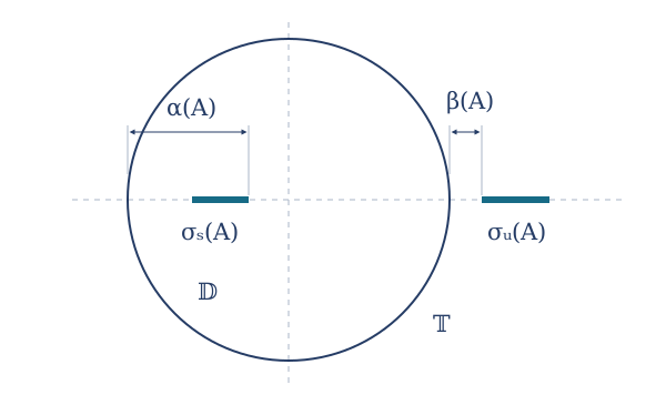
Spectral picture of a normal hyperbolic operator with both spectral components present. The unit circle separates the stable part \(\sigma_s(A)=\sigma(A)\cap\mathbb{D}\) from the unstable part \(\sigma_u(A)\). The two gap parameters \(\alpha(A)=1-\rho_s(A)\) and \(\beta(A)=\rho_u(A)-1\) measure the distances of the two components from the unit circle; the hyperbolicity margin equals the smaller of them, \(r_{\mathrm{hyp}}(A)=\min\{\alpha(A),\beta(A)\}\).
The geometry behind (1.1) is specifically Hilbertian; see Figure 1 for the spectral configuration underlying the two gap parameters. For a normal operator, the stable and unstable spectral subspaces form an orthogonal decomposition. The two components of the Green operator can therefore be combined quadratically rather than by a triangle inequality. This immediately suggests the upper estimate in (1.1), but sharpness requires an additional argument. We construct a bounded forcing whose negative-time part asymptotically maximizes the stable response and whose nonnegative-time part asymptotically maximizes the unstable response. Approximate eigenvectors associated with the two extremal spectral points align the corresponding finite Green sums. Since the two forcing components occupy disjoint time intervals, they can be combined without increasing the \(\ell^\infty\) norm of the forcing. The quantitative statement is thus considerably finer than the qualitative one: the identity (1.1) describes how the optimal amplification degenerates as the spectrum approaches the unit circle. In this sense, it provides a quantitative refinement of the qualitative hyperbolicity–shadowing equivalence for normal operators established in [7].
The second main result relates the exact shadowability constant to the robustness of hyperbolicity. We first show that for an arbitrary hyperbolic operator
\[\operatorname{Shad}(A) \ge \frac{1}{r_{\mathrm{hyp}}(A)}. \tag{1.2}\]
For normal operators the spectral theorem gives an explicit expression for the hyperbolicity margin. In the mixed stable–unstable case, \[r_{\mathrm{hyp}}(A) = \min\{\alpha(A),\beta(A)\}.\] Combining this identity with (1.1) yields
\[r_{\mathrm{hyp}}(A)\operatorname{Shad}(A) = \left(1+\eta(A)^2\right)^{1/2}, \tag{1.3}\]
where \[\eta(A):= \frac{\min\{\alpha(A),\beta(A)\}} {\max\{\alpha(A),\beta(A)\}}.\] Consequently,
\[1 \le r_{\mathrm{hyp}}(A)\operatorname{Shad}(A) \le \sqrt{2}. \tag{1.4}\]
The upper constant \(\sqrt{2}\) is attained precisely when the stable and unstable spectral gaps are equal. The lower value \(1\) is attained in the one-sided stable and unstable cases, while the inequality is strict on the left whenever both spectral components are nonempty.
Thus the normalized shadowability constant is governed by the relative balance of the stable and unstable spectral gaps rather than by their absolute size alone.
Two features of the quantitative theory deserve emphasis at the outset. First, the right-hand side of (1.1) is the norm of the inverse of the difference operator \(\mathcal L_A\), whereas a qualitative shadowing statement for hyperbolic operators produces only the existence of a bounded solution and hence an unspecified finite constant. Second, the difference operator treats past and future asymmetrically, so that the two one-sided cases in Corollary 3.2 have to be treated separately.
The paper is organized as follows. In Section 2 we introduce the notation used throughout the paper, recall the difference-operator formulation of uniform linear shadowing, and establish the basic relation between the shadowability constant and the hyperbolicity margin. Section 3 contains the exact computation of the shadowability constant for normal hyperbolic operators. In Section 4 we derive the sharp stability ratio (1.4), characterize the equality cases, and give examples showing that the constants cannot be improved, including an infinite-dimensional example whose spectra have no spectral-edge eigenvalues. Section 5 contains concluding remarks and indicates possible extensions beyond the normal setting.
2. Preliminaries and Hyperbolicity Margins
Throughout the paper, \(H\) denotes a complex Hilbert space with norm \(\|\cdot\|\), and \(\mathcal{B}(H)\) denotes the Banach algebra of all bounded linear operators on \(H\), equipped with the operator norm, which is also denoted by \(\|\cdot\|\). The identity operator on \(H\) is denoted by \(I\). For \(A\in\mathcal{B}(H)\), its spectrum is denoted by \(\sigma(A)\).
We write \[\mathbb{D}:=\{z\in\mathbb{C}:|z|<1\}, \qquad \mathbb{T}:=\{z\in\mathbb{C}:|z|=1\}.\] An operator \(A\in\mathcal{B}(H)\) is called hyperbolic if
\[\sigma(A)\cap\mathbb{T}=\varnothing. \tag{2.1}\]
In what follows, whenever bi-infinite dynamics are considered, the operator \(A\) is assumed to be invertible.
For a hyperbolic operator \(A\), define the stable and unstable parts of the spectrum by
\[\begin{aligned} \sigma_s(A)&:=\sigma(A)\cap\mathbb{D},\\ \sigma_u(A)&:=\sigma(A)\cap\{z\in\mathbb{C}:|z|>1\}. \end{aligned} \tag{2.2}\]
Since \(\sigma(A)\) is compact and disjoint from \(\mathbb{T}\), these two sets are disjoint compact spectral subsets and \[\sigma(A)=\sigma_s(A)\cup\sigma_u(A).\]
Let \(P_s\) and \(P_u\) denote the Riesz spectral projections associated with \(\sigma_s(A)\) and \(\sigma_u(A)\), respectively. We set
\[H_s:=P_sH, \qquad H_u:=P_uH, \tag{2.3}\]
and denote the corresponding restrictions of \(A\) by
\[A_s:=A|_{H_s}, \qquad A_u:=A|_{H_u}. \tag{2.4}\]
Then \[H=H_s\oplus H_u,\] and both \(H_s\) and \(H_u\) are invariant under \(A\). If \(A\) is normal, the spectral theorem [17] implies that \(H_s\) and \(H_u\) are reducing and orthogonal. In that case,
\[H=H_s\oplus^\perp H_u, \qquad P_s=P_s^*, \qquad P_u=P_u^*. \tag{2.5}\]
Whenever \(\sigma_s(A)\neq\varnothing\), we define
\[\rho_s(A) := \max_{\lambda\in\sigma_s(A)}|\lambda|, \qquad \alpha(A):=1-\rho_s(A). \tag{2.6}\]
Similarly, whenever \(\sigma_u(A)\neq\varnothing\), we define
\[\rho_u(A) := \min_{\lambda\in\sigma_u(A)}|\lambda|, \qquad \beta(A):=\rho_u(A)-1. \tag{2.7}\]
Hyperbolicity implies \[0<\alpha(A), \qquad 0<\beta(A)\] whenever the corresponding spectral component is nonempty. For brevity, when the operator is fixed we write \[\rho_s,\quad \rho_u,\quad \alpha,\quad \beta\] instead of \[\rho_s(A),\quad \rho_u(A),\quad \alpha(A),\quad \beta(A).\]
The difference operator and the shadowability constant
Let \[\ell^\infty(\mathbb{Z},H) := \left\{ x=(x_n)_{n\in\mathbb{Z}}: \sup_{n\in\mathbb{Z}}\|x_n\|<\infty \right\},\] equipped with the norm
\[\|x\|_\infty := \sup_{n\in\mathbb{Z}}\|x_n\|. \tag{2.8}\]
For \(A\in\mathcal{B}(H)\), define the difference operator \[\mathcal L_A: \ell^\infty(\mathbb{Z},H)\longrightarrow\ell^\infty(\mathbb{Z},H)\] by
\[(\mathcal L_Ax)_n := x_{n+1}-Ax_n, \qquad n\in\mathbb{Z}. \tag{2.9}\]
Following Morales and Nguyen [11], the shadowability constant of an invertible linear operator \(A\) is denoted by \(\operatorname{Shad}(A)\). Equivalently, \(\operatorname{Shad}(A)\) is the infimum of all constants \(K>0\) with the following property: for every \(e=(e_n)_{n\in\mathbb{Z}}\in\ell^\infty(\mathbb{Z},H)\) there exists \(x=(x_n)_{n\in\mathbb{Z}}\in\ell^\infty(\mathbb{Z},H)\) satisfying
\[x_{n+1}-Ax_n=e_n, \qquad n\in\mathbb{Z}, \tag{2.10}\]
and
\[\|x\|_\infty \le K\|e\|_\infty. \tag{2.11}\]
For hyperbolic \(A\), the difference operator \(\mathcal L_A\) is invertible and
\[\operatorname{Shad}(A) = \|\mathcal L_A^{-1}\|_{\mathcal{B}(\ell^\infty(\mathbb{Z},H))}. \tag{2.12}\]
Indeed, \(\mathcal L_A\) is bijective by Lemma 2.1 below, so its inverse is bounded by the open mapping theorem, and (2.12) merely restates the definition of the operator norm together with the scale invariance of (2.11). We shall use (2.12) throughout the paper.
The inverse of \(\mathcal L_A\) admits the usual Green representation. For completeness, we record the formula in the notation used here.
Lemma 2.1
Let \(A\in\mathcal{B}(H)\) be invertible and hyperbolic. For every \(e=(e_n)_{n\in\mathbb{Z}}\in\ell^\infty(\mathbb{Z},H)\), the unique bounded solution of (2.10) is given by
\[\begin{aligned} (\mathcal L_A^{-1}e)_n &= \sum_{j=0}^{\infty} A_s^jP_se_{n-1-j}\\ &\quad - \sum_{j=0}^{\infty} A_u^{-j-1}P_ue_{n+j}, \qquad n\in\mathbb{Z}. \end{aligned} \tag{2.13}\]
Both series converge in \(H\), uniformly with respect to \(n\) for \(e\) ranging over bounded subsets of \(\ell^\infty(\mathbb{Z},H)\).
Proof.
Since \[\sigma(A_s)\subset\mathbb{D}, \qquad \sigma(A_u^{-1})\subset\mathbb{D},\] we have \[r(A_s)<1, \qquad r(A_u^{-1})<1,\] where \(r(\cdot)\) denotes the spectral radius. Choose numbers \(q_s,q_u\in(0,1)\) satisfying \[r(A_s)<q_s<1, \qquad r(A_u^{-1})<q_u<1.\] By the spectral radius formula, there exist constants \(C_s,C_u>0\) such that \[\|A_s^j\|\le C_sq_s^j, \qquad \|A_u^{-j}\|\le C_uq_u^j, \qquad j\ge0.\] Hence both series in (2.13) converge absolutely and uniformly in \(n\) whenever \(\|e\|_\infty\) is bounded.
Set \[x_n^s := \sum_{j=0}^{\infty}A_s^jP_se_{n-1-j}.\] Then \[x_{n+1}^s = P_se_n + \sum_{j=1}^{\infty}A_s^jP_se_{n-j},\] whereas \[A_sx_n^s = \sum_{j=1}^{\infty}A_s^jP_se_{n-j}.\] Therefore
\[x_{n+1}^s-A_sx_n^s=P_se_n. \tag{2.14}\]
Similarly, define \[x_n^u := - \sum_{j=0}^{\infty}A_u^{-j-1}P_ue_{n+j}.\] A direct index shift gives
\[x_{n+1}^u-A_ux_n^u=P_ue_n. \tag{2.15}\]
Since \(P_s+P_u=I\), adding (2.14) and (2.15) yields \[x_{n+1}-Ax_n=e_n,\] where \(x_n=x_n^s+x_n^u\).
It remains to prove uniqueness. Suppose that \(y=(y_n)_{n\in\mathbb{Z}}\in\ell^\infty(\mathbb{Z},H)\) satisfies \[y_{n+1}=Ay_n, \qquad n\in\mathbb{Z}.\] Write \(y_n=y_n^s+y_n^u\), where \(y_n^s=P_sy_n\) and \(y_n^u=P_uy_n\). For every \(m\ge0\), \[y_0^s=A_s^m y_{-m}^s.\] Hence \[\|y_0^s\| \le C_sq_s^m\|y\|_\infty.\] Letting \(m\to\infty\) gives \(y_0^s=0\). Similarly, \[y_0^u=A_u^{-m}y_m^u,\] and therefore \[\|y_0^u\| \le C_uq_u^m\|y\|_\infty\longrightarrow0.\] Thus \(y_0=0\), and consequently \(y_n=0\) for every \(n\in\mathbb{Z}\).
□
Remark 2.2
Formula (2.13) exhibits an asymmetry that will be crucial in Section 3: at a fixed time \(n\), the stable component of the bounded response depends only on the forcing at times strictly smaller than \(n\), whereas the unstable component depends only on the forcing at times greater than or equal to \(n\). This separation allows the two components to be optimized simultaneously under a single \(\ell^\infty\) constraint.
The hyperbolicity margin
We now introduce the second quantitative object considered in this paper.
Definition 2.3
Let \(A\in\mathcal{B}(H)\) be hyperbolic. The hyperbolicity margin of \(A\) is
\[r_{\mathrm{hyp}}(A) := \inf \bigl\{ \|E\|: E\in\mathcal{B}(H),\, \sigma(A+E)\cap\mathbb{T}\neq\varnothing \bigr\}. \tag{2.16}\]
Thus \(r_{\mathrm{hyp}}(A)\) is the operator-norm distance from \(A\) to the complement of the set of hyperbolic operators. The following resolvent characterization is standard in stability-radius theory; see, e.g., [18]. We include the short proof for completeness.
Proposition 2.4
Let \(A\in\mathcal{B}(H)\) be hyperbolic. Then
\[r_{\mathrm{hyp}}(A) = \left( \max_{z\in\mathbb{T}} \|(zI-A)^{-1}\| \right)^{-1}. \tag{2.17}\]
Proof.
We first recall that if \(B\in\mathcal{B}(H)\) is invertible, then
\[\operatorname{dist}\bigl( B,\mathcal{B}(H)\setminus GL(H) \bigr) = \frac{1}{\|B^{-1}\|}, \tag{2.18}\]
where \(GL(H)\) denotes the group of bounded invertible operators on \(H\).
Indeed, if \(F\in\mathcal{B}(H)\) satisfies \[\|F\|<\|B^{-1}\|^{-1},\] then \[B+F=B(I+B^{-1}F)\] is invertible by the Neumann series. Hence the left-hand side of (2.18) is at least \(\|B^{-1}\|^{-1}\).
For the reverse inequality, set \[m(B):=\inf_{\|x\|=1}\|Bx\|.\] Since \(B\) is invertible, \[m(B)=\|B^{-1}\|^{-1}.\] Given \(\varepsilon>0\), choose a unit vector \(x_\varepsilon\in H\) such that \[\|Bx_\varepsilon\| < m(B)+\varepsilon.\] Define the rank-one operator \(F_\varepsilon\in\mathcal{B}(H)\) by \[F_\varepsilon x := -\langle x,x_\varepsilon\rangle Bx_\varepsilon, \qquad x\in H.\] Then \[(B+F_\varepsilon)x_\varepsilon=0,\] so \(B+F_\varepsilon\) is not invertible. Moreover, \(F_\varepsilon x=-\langle x,x_\varepsilon\rangle Bx_\varepsilon\), so Cauchy–Schwarz gives \(\|F_\varepsilon\|\le\|Bx_\varepsilon\|\), while testing \(F_\varepsilon\) on \(x_\varepsilon\) gives the reverse inequality. Hence \[\|F_\varepsilon\| = \|Bx_\varepsilon\| < \|B^{-1}\|^{-1}+\varepsilon.\] Letting \(\varepsilon\downarrow0\) proves (2.18).
Now fix \(z\in\mathbb{T}\). Since \(A\) is hyperbolic, \(zI-A\) is invertible. The condition \[z\in\sigma(A+E)\] is equivalent to the noninvertibility of \[zI-A-E.\] Applying (2.18) to \(B=zI-A\) shows that \[\inf\{ \|E\|: z\in\sigma(A+E) \} = \frac{1}{\|(zI-A)^{-1}\|},\] since \(z\in\sigma(A+E)\) if and only if \((zI-A)-E\) is not invertible. Taking the infimum over \(z\in\mathbb{T}\) yields \[r_{\mathrm{hyp}}(A) = \inf_{z\in\mathbb{T}} \frac{1}{\|(zI-A)^{-1}\|}.\] The map \[z\longmapsto(zI-A)^{-1}\] is norm-continuous on the compact set \(\mathbb{T}\). Hence the continuous positive function \(z\mapsto\|(zI-A)^{-1}\|\) attains a maximum there, and taking reciprocals turns that maximum into the minimum of \(z\mapsto\|(zI-A)^{-1}\|^{-1}\). Therefore \[r_{\mathrm{hyp}}(A) = \left( \max_{z\in\mathbb{T}} \|(zI-A)^{-1}\| \right)^{-1}.\]
□
The resolvent characterization immediately gives a universal lower bound for the shadowability constant.
Proposition 2.5
Let \(A\in\mathcal{B}(H)\) be invertible and hyperbolic. Then
\[\operatorname{Shad}(A) \ge \frac{1}{r_{\mathrm{hyp}}(A)}. \tag{2.19}\]
Equivalently,
\[r_{\mathrm{hyp}}(A)\operatorname{Shad}(A)\ge1. \tag{2.20}\]
Proof.
Fix \(z\in\mathbb{T}\) and a nonzero vector \(v\in H\). Define \(e=(e_n)_{n\in\mathbb{Z}}\in\ell^\infty(\mathbb{Z},H)\) by \[e_n:=z^nv, \qquad n\in\mathbb{Z}.\] Since \(|z|=1\), \[\|e\|_\infty=\|v\|.\] Define \[x_n := z^n(zI-A)^{-1}v, \qquad n\in\mathbb{Z}.\] Then \(x\in\ell^\infty(\mathbb{Z},H)\) and \[\begin{aligned} x_{n+1}-Ax_n &= z^{n+1}(zI-A)^{-1}v - Az^n(zI-A)^{-1}v\\ &= z^n(zI-A)(zI-A)^{-1}v = z^nv = e_n. \end{aligned}\] Thus, by (2.12), \[\operatorname{Shad}(A) \ge \frac{\|x\|_\infty}{\|e\|_\infty} = \frac{\|(zI-A)^{-1}v\|}{\|v\|}.\] Taking the supremum over all \(v\neq0\) gives \[\operatorname{Shad}(A) \ge \|(zI-A)^{-1}\|.\] Since this holds for every \(z\in\mathbb{T}\), \[\operatorname{Shad}(A) \ge \max_{z\in\mathbb{T}}\|(zI-A)^{-1}\|.\] Proposition 2.4 now gives (2.19).
□
Remark 2.6
Proposition 2.5 does not require normality. It shows that the reciprocal hyperbolicity margin is a universal lower bound for uniform shadowing amplification. The normal case considered in the next section is distinguished by the fact that the gap between these two quantities can be determined exactly.
3. Sharp Shadowability Bounds for Normal Hyperbolic Operators
We now assume that \(A\in\mathcal{B}(H)\) is normal, invertible and hyperbolic. The orthogonality of the stable and unstable spectral subspaces makes it possible to sharpen the general Green-operator estimate to an exact formula.
We begin with the mixed case, in which \[\sigma_s(A)\neq\varnothing \qquad\text{and}\qquad \sigma_u(A)\neq\varnothing.\] Recall from (2.6) and (2.7) that \[\rho_s = \max_{\lambda\in\sigma_s(A)}|\lambda|, \qquad \alpha=1-\rho_s,\] and \[\rho_u = \min_{\lambda\in\sigma_u(A)}|\lambda|, \qquad \beta=\rho_u-1.\]
Theorem 3.1
Let \(H\) be a complex Hilbert space and let \(A\in\mathcal{B}(H)\) be an invertible normal hyperbolic operator. Suppose that both \(\sigma_s(A)\) and \(\sigma_u(A)\) are nonempty. Then
\[\boxed{ \operatorname{Shad}(A) = \left( \alpha^{-2}+\beta^{-2} \right)^{1/2}. } \tag{3.1}\]
Proof.
We divide the proof into the upper and lower estimates.
Step 1: the upper estimate. Let \[e=(e_n)_{n\in\mathbb{Z}}\in\ell^\infty(\mathbb{Z},H)\] and put \[x:=\mathcal L_A^{-1}e.\] By Lemma 2.1, \[x_n=x_n^s+x_n^u,\] where
\[x_n^s := \sum_{j=0}^{\infty}A_s^jP_se_{n-1-j} \in H_s \tag{3.2}\]
and
\[x_n^u := - \sum_{j=0}^{\infty}A_u^{-j-1}P_ue_{n+j} \in H_u. \tag{3.3}\]
Since \(A\) is normal, \(H_s\perp H_u\). Hence
\[\|x_n\|^2 = \|x_n^s\|^2+\|x_n^u\|^2. \tag{3.4}\]
The restrictions \(A_s\) and \(A_u\) are normal. By the spectral theorem, \[\|A_s^j\| = \rho_s^j, \qquad j\ge0.\]
Moreover, \(P_s\) is an orthogonal projection, so \(\|P_s\|=1\). Consequently, \[\begin{aligned} \|x_n^s\| &\le \sum_{j=0}^{\infty} \|A_s^j\|\,\|P_se_{n-1-j}\|\\ &\le \sum_{j=0}^{\infty}\rho_s^j\|e\|_\infty\\ &= \frac{1}{1-\rho_s}\|e\|_\infty = \frac{1}{\alpha}\|e\|_\infty. \end{aligned}\] Similarly, since \(A_u^{-1}\) is normal and \[\|A_u^{-1}\|=\rho_u^{-1},\] we have \[\|A_u^{-j-1}\| = \rho_u^{-j-1}, \qquad j\ge0.\] Thus \[\begin{aligned} \|x_n^u\| &\le \sum_{j=0}^{\infty} \rho_u^{-j-1}\|e\|_\infty\\ &= \frac{1}{\rho_u-1}\|e\|_\infty = \frac{1}{\beta}\|e\|_\infty. \end{aligned}\] Combining these estimates with (3.4), we obtain \[\|x_n\|^2 \le \left( \alpha^{-2}+\beta^{-2} \right)\|e\|_\infty^2\] for every \(n\in\mathbb{Z}\). Therefore
\[\operatorname{Shad}(A) \le \left( \alpha^{-2}+\beta^{-2} \right)^{1/2}. \tag{3.5}\]
Step 2: approximate eigenvectors at the edge. Since \(\sigma_s(A)\) and \(\sigma_u(A)\) are compact and nonempty, there exist \[\lambda_s\in\sigma_s(A), \qquad \lambda_u\in\sigma_u(A)\] such that \[|\lambda_s|=\rho_s, \qquad |\lambda_u|=\rho_u.\] Write
\[\lambda_s=\rho_se^{i\theta_s}, \qquad \lambda_u=\rho_ue^{i\theta_u}, \tag{3.6}\]
where \(\theta_s,\theta_u\in[0,2\pi)\).
For a bounded normal operator, every spectral value belongs to its approximate point spectrum [17]. Applied to the normal restrictions \(A_s\) and \(A_u\), this yields sequences of unit vectors \[(v_{s,k})_{k\ge1}\subset H_s, \qquad (v_{u,k})_{k\ge1}\subset H_u\] such that
\[\|(A_s-\lambda_sI)v_{s,k}\| \longrightarrow0 \tag{3.7}\]
and
\[\|(A_u-\lambda_uI)v_{u,k}\| \longrightarrow0 \tag{3.8}\]
as \(k\to\infty\).
Fix an integer \(N\ge0\). For every \(0\le j\le N\), the identity \[A_s^j-\lambda_s^jI = \sum_{\ell=0}^{j-1} \lambda_s^{\,j-1-\ell} A_s^\ell(A_s-\lambda_sI)\] implies, by (3.7), that
\[\max_{0\le j\le N} \| (A_s^j-\lambda_s^jI)v_{s,k} \| \longrightarrow0. \tag{3.9}\]
For the unstable component, observe that \[A_u^{-1}-\lambda_u^{-1}I = -\lambda_u^{-1} A_u^{-1}(A_u-\lambda_uI).\] Hence (3.8) gives \[\| (A_u^{-1}-\lambda_u^{-1}I)v_{u,k} \| \longrightarrow0.\] Applying the preceding finite-power argument to \(A_u^{-1}\) yields
\[\max_{1\le m\le N+1} \| (A_u^{-m}-\lambda_u^{-m}I)v_{u,k} \| \longrightarrow0. \tag{3.10}\]
Step 3: a past–future forcing. For each \(k\ge1\), define \[e^{(N,k)} = (e_n^{(N,k)})_{n\in\mathbb{Z}} \in\ell^\infty(\mathbb{Z},H)\] by
\[\begin{aligned} e_n^{(N,k)} &:= e^{-ij\theta_s}v_{s,k}, \qquad n=-1-j,\quad 0\le j\le N,\\ e_n^{(N,k)} &:= e^{i(j+1)\theta_u}v_{u,k}, \qquad n=j,\quad 0\le j\le N,\\ e_n^{(N,k)} &:= 0, \qquad\text{otherwise}. \end{aligned} \tag{3.11}\]
The two nonzero parts in (3.11) have disjoint time supports, and all nonzero entries are unit vectors. Therefore
\[\|e^{(N,k)}\|_\infty=1. \tag{3.12}\]
Let \[x^{(N,k)} := \mathcal L_A^{-1}e^{(N,k)}.\] At time \(n=0\), the Green representation gives \[x_0^{(N,k)} = s_{N,k}-u_{N,k},\] where
\[s_{N,k} := \sum_{j=0}^{N} e^{-ij\theta_s}A_s^jv_{s,k} \in H_s \tag{3.13}\]
and
\[u_{N,k} := \sum_{j=0}^{N} e^{i(j+1)\theta_u}A_u^{-j-1}v_{u,k} \in H_u. \tag{3.14}\]
\[\left\| s_{N,k} - \left( \sum_{j=0}^{N}\rho_s^j \right)v_{s,k} \right\| \longrightarrow0 \qquad(k\to\infty). \tag{3.15}\]
Likewise, by (3.10),
\[\left\| u_{N,k} - \left( \sum_{j=0}^{N}\rho_u^{-j-1} \right)v_{u,k} \right\| \longrightarrow0. \tag{3.16}\]
Since \(s_{N,k}\in H_s\), \(u_{N,k}\in H_u\), and \(H_s\perp H_u\), \[\|x_0^{(N,k)}\|^2 = \|s_{N,k}\|^2+\|u_{N,k}\|^2.\] Using (3.15) and (3.16), and recalling that \(\|v_{s,k}\|=\|v_{u,k}\|=1\), we obtain \[\lim_{k\to\infty} \|x_0^{(N,k)}\|^2 = \left( \sum_{j=0}^{N}\rho_s^j \right)^2 + \left( \sum_{j=0}^{N}\rho_u^{-j-1} \right)^2.\] By (3.12) and the definition of \(\operatorname{Shad}(A)\), \[\operatorname{Shad}(A) \ge \|x^{(N,k)}\|_\infty \ge \|x_0^{(N,k)}\|.\] Letting \(k\to\infty\) therefore gives
\[\operatorname{Shad}(A)^2 \ge \left( \sum_{j=0}^{N}\rho_s^j \right)^2 + \left( \sum_{j=0}^{N}\rho_u^{-j-1} \right)^2. \tag{3.17}\]
Finally, letting \(N\to\infty\) in (3.17) yields \[\operatorname{Shad}(A)^2 \ge \frac{1}{(1-\rho_s)^2} + \frac{1}{(\rho_u-1)^2} = \alpha^{-2}+\beta^{-2}.\] Thus
\[\operatorname{Shad}(A) \ge \left( \alpha^{-2}+\beta^{-2} \right)^{1/2}. \tag{3.18}\]
Combining (3.5) and (3.18) proves (3.1).
□
Corollary 3.2
Let \(H\) be a complex Hilbert space and let \(A\in\mathcal{B}(H)\) be an invertible normal hyperbolic operator.
If \(\sigma_u(A)=\varnothing\), then
\[\operatorname{Shad}(A) = \frac{1}{\alpha(A)}. \tag{3.19}\]
If \(\sigma_s(A)=\varnothing\), then
\[\operatorname{Shad}(A) = \frac{1}{\beta(A)}. \tag{3.20}\]
Proof.
We prove only the stable case, since the unstable case is analogous. If \(\sigma_u(A)=\varnothing\), then \(H=H_s\) and the Green representation reduces to \[(\mathcal L_A^{-1}e)_n = \sum_{j=0}^{\infty}A^je_{n-1-j}.\] Normality gives \(\|A^j\|=\rho_s(A)^j\), and therefore \[\operatorname{Shad}(A)\le\frac{1}{1-\rho_s(A)}=\frac{1}{\alpha(A)}.\] The reverse inequality follows from the same finite, phase-aligned approximate eigenvector construction used in the proof of Theorem 3.1, with the unstable forcing omitted. Hence \[\operatorname{Shad}(A)=\frac{1}{\alpha(A)}.\] The purely unstable case is analogous to the stable one. If \(\sigma_s(A)=\varnothing\), the Green representation becomes \[(\mathcal L_A^{-1}e)_n = - \sum_{j=0}^{\infty}A^{-j-1}e_{n+j}.\] Since \(A^{-1}\) is normal and \[\|A^{-1}\|=\rho_u(A)^{-1},\] we obtain \[\operatorname{Shad}(A) \le \sum_{j=0}^{\infty}\rho_u(A)^{-j-1} = \frac{1}{\rho_u(A)-1} = \frac{1}{\beta(A)}.\] For the reverse inequality, choose \(\lambda_u\in\sigma(A)\) such that \(|\lambda_u|=\rho_u(A)\) and write \(\lambda_u=\rho_u(A)e^{i\theta_u}\). Using unit approximate eigenvectors associated with \(\lambda_u\) and the finite future forcing \[e_j=e^{i(j+1)\theta_u}v_k, \qquad 0\le j\le N,\] with \(e_j=0\) otherwise, the argument in Step 3 of Theorem 3.1 gives \[\operatorname{Shad}(A) \ge \sum_{j=0}^{N}\rho_u(A)^{-j-1}.\] Letting \(N\to\infty\) yields \[\operatorname{Shad}(A) \ge \frac{1}{\rho_u(A)-1} = \frac{1}{\beta(A)}.\] Therefore \[\operatorname{Shad}(A)=\frac{1}{\beta(A)}.\]
□
Remark 3.3
In the mixed case, Theorem 3.1 gives the Euclidean combination \[\operatorname{Shad}(A) = \left( \alpha^{-2}+\beta^{-2} \right)^{1/2},\] rather than the additive estimate \[\alpha^{-1}+\beta^{-1}.\] The additive expression is what one obtains for a general Banach-space splitting \(X=S\oplus U\): the estimate \(\operatorname{Shad}(A)\le\sum_{k\ge0}\|A^k|_S\|+\sum_{k\ge1}\|A^{-k}|_U\|\) of [11, Theorem 8], applied to the hyperbolic splitting of a normal operator and combined with \(\|A^k|_S\|=\rho_s^k\) and \(\|A^{-k}|_U\|=\rho_u^{-k}\), yields exactly \(\alpha^{-1}+\beta^{-1}\). The improvement to (3.1) is thus a direct consequence of two facts specific to the present setting: the stable and unstable subspaces are orthogonal, and their extremal responses can be generated by forcing supported on disjoint parts of the time axis.
4. Stability Ratios and Sharpness
We now combine the exact shadowability formula with the hyperbolicity margin introduced in Definition 2.3.
We first identify the latter explicitly in the normal case.
Proposition 4.1
Let \(H\) be a complex Hilbert space and let \(A\in\mathcal{B}(H)\) be a normal hyperbolic operator. Then
\[r_{\mathrm{hyp}}(A) = \operatorname{dist}(\sigma(A),\mathbb{T}), \tag{4.1}\]
where \[\operatorname{dist}(\sigma(A),\mathbb{T}) := \inf\{ |\lambda-z|: \lambda\in\sigma(A),\ z\in\mathbb{T} \}.\] In particular, if both \(\sigma_s(A)\) and \(\sigma_u(A)\) are nonempty, then
\[r_{\mathrm{hyp}}(A) = \min\{\alpha(A),\beta(A)\}. \tag{4.2}\]
If \(\sigma_u(A)=\varnothing\), then
\[r_{\mathrm{hyp}}(A)=\alpha(A), \tag{4.3}\]
while if \(\sigma_s(A)=\varnothing\), then
\[r_{\mathrm{hyp}}(A)=\beta(A). \tag{4.4}\]
Proof.
For a normal operator and every \(z\notin\sigma(A)\), the spectral theorem gives
\[\|(zI-A)^{-1}\| = \frac{1}{\operatorname{dist}(z,\sigma(A))}, \tag{4.5}\]
where \[\operatorname{dist}(z,\sigma(A)) := \inf_{\lambda\in\sigma(A)}|z-\lambda|.\] Combining (4.5) with Proposition 2.4, we obtain \[\begin{aligned} r_{\mathrm{hyp}}(A) &= \left( \max_{z\in\mathbb{T}} \frac{1}{\operatorname{dist}(z,\sigma(A))} \right)^{-1}\\ &= \min_{z\in\mathbb{T}}\operatorname{dist}(z,\sigma(A))\\ &= \operatorname{dist}(\sigma(A),\mathbb{T}). \end{aligned}\] This proves (4.1).
Suppose now that both spectral components are nonempty. For \(\lambda\in\mathbb{C}\), \[\operatorname{dist}(\lambda,\mathbb{T}) = \bigl||\lambda|-1\bigr|.\] Hence \[\operatorname{dist}(\sigma_s(A),\mathbb{T}) = 1-\rho_s(A) = \alpha(A),\] and \[\operatorname{dist}(\sigma_u(A),\mathbb{T}) = \rho_u(A)-1 = \beta(A).\] Since \[\sigma(A)=\sigma_s(A)\cup\sigma_u(A),\] it follows that \[r_{\mathrm{hyp}}(A) = \min\{\alpha(A),\beta(A)\}.\] The one-sided cases follow in the same way.
□
We can now state the second main theorem.
Theorem 4.2
Let \(H\) be a complex Hilbert space and let \(A\in\mathcal{B}(H)\) be an invertible normal hyperbolic operator. Then
\[\boxed{ 1 \le r_{\mathrm{hyp}}(A)\operatorname{Shad}(A) \le \sqrt{2}. } \tag{4.6}\]
Both constants in (4.6) are optimal.
If both \(\sigma_s(A)\) and \(\sigma_u(A)\) are nonempty, then
\[\boxed{ r_{\mathrm{hyp}}(A)\operatorname{Shad}(A) = \left[ 1+ \left( \frac{\min\{\alpha(A),\beta(A)\}} {\max\{\alpha(A),\beta(A)\}} \right)^{\!2}\, \right]^{\!1/2}. } \tag{4.7}\]
Consequently,
\[1 < r_{\mathrm{hyp}}(A)\operatorname{Shad}(A) \le \sqrt{2} \tag{4.8}\]
in the mixed case, and equality in the upper bound holds if and only if
\[\alpha(A)=\beta(A). \tag{4.9}\]
If the spectrum is one-sided, then
\[r_{\mathrm{hyp}}(A)\operatorname{Shad}(A)=1. \tag{4.10}\]
Proof.
Suppose first that both spectral components are nonempty. By Theorem 3.1 and Proposition 4.1, \[\operatorname{Shad}(A) = \left( \alpha(A)^{-2}+\beta(A)^{-2} \right)^{1/2}\] and \[r_{\mathrm{hyp}}(A)=\min\{\alpha(A),\beta(A)\}.\] Set \[\begin{aligned} m&:=\min\{\alpha(A),\beta(A)\},\\ M&:=\max\{\alpha(A),\beta(A)\}. \end{aligned}\]
Then \[0<m\le M,\] and \[\begin{aligned} r_{\mathrm{hyp}}(A)\operatorname{Shad}(A) &= m \left( \alpha(A)^{-2}+\beta(A)^{-2} \right)^{1/2}\\ &= \left( 1+\frac{m^2}{M^2} \right)^{1/2}. \end{aligned}\] This proves (4.7).
Since \[0<\frac{m}{M}\le1,\] we obtain \[1 < \left( 1+\frac{m^2}{M^2} \right)^{1/2} \le \sqrt2.\] The upper equality holds precisely when \[m=M,\] which is equivalent to \[\alpha(A)=\beta(A).\]
Now suppose that \(\sigma_u(A)=\varnothing\). By Corollary 3.2 and Proposition 4.1, \[\operatorname{Shad}(A)=\frac1{\alpha(A)}, \qquad r_{\mathrm{hyp}}(A)=\alpha(A),\] and hence \[r_{\mathrm{hyp}}(A)\operatorname{Shad}(A)=1.\] The purely unstable case is identical, using \[\operatorname{Shad}(A)=\frac1{\beta(A)} \qquad\text{and}\qquad r_{\mathrm{hyp}}(A)=\beta(A).\] Thus (4.6) holds in all cases.
□
Remark 4.3
In the mixed case, define the spectral-balance parameter
\[\eta(A) := \frac{\min\{\alpha(A),\beta(A)\}} {\max\{\alpha(A),\beta(A)\}} \in(0,1]. \tag{4.11}\]
Then Theorem 4.2 may be written in the compact form
\[r_{\mathrm{hyp}}(A)\operatorname{Shad}(A) = \sqrt{1+\eta(A)^2}. \tag{4.12}\]
Thus the normalized shadowability constant is determined entirely by the relative balance of the two spectral gaps.
We next give two examples illustrating the equality cases.
Example 4.4 — The lower constant
Let \(0<r<1\) and let \[A=rI\] on any nonzero complex Hilbert space \(H\). Then \(A\) is normal, invertible and purely stable. We have \[\rho_s(A)=r, \qquad \alpha(A)=1-r.\] Hence \[\operatorname{Shad}(A)=\frac{1}{1-r}\] and \[r_{\mathrm{hyp}}(A)=1-r.\] Therefore \[r_{\mathrm{hyp}}(A)\operatorname{Shad}(A)=1.\] Thus the lower constant in (4.6) is attained.
Example 4.5 — A balanced finite-dimensional model
Let \(0<\varepsilon<1\) and consider \[A_\varepsilon = \begin{pmatrix} 1-\varepsilon & 0\\ 0 & 1+\varepsilon \end{pmatrix}\] acting on \(\mathbb{C}^2\) with its standard Hilbert norm. Then \(A_\varepsilon\) is normal, invertible and hyperbolic, with \[\alpha(A_\varepsilon) = \beta(A_\varepsilon) = \varepsilon.\] Therefore \[\operatorname{Shad}(A_\varepsilon) = \frac{\sqrt2}{\varepsilon}, \qquad r_{\mathrm{hyp}}(A_\varepsilon) = \varepsilon,\] and hence \[r_{\mathrm{hyp}}(A_\varepsilon)\operatorname{Shad}(A_\varepsilon) = \sqrt2.\] Thus the upper constant in (4.6) is already sharp in dimension two.
The next example shows that the upper constant remains sharp in an infinite-dimensional setting with continuous spectrum.
Example 4.6 — Continuous spectrum and sharpness
Let \[H = L^2([0,1]) \oplus L^2([0,1]),\] and fix \[0<\varepsilon<\frac14.\] Define \[A_\varepsilon = M_{s,\varepsilon} \oplus M_{u,\varepsilon},\] where \[(M_{s,\varepsilon}f)(t) := \left( 1-\varepsilon-\frac{t}{4} \right)f(t), \qquad f\in L^2([0,1]),\] and \[(M_{u,\varepsilon}g)(t) := \left( 1+\varepsilon+\frac{t}{4} \right)g(t), \qquad g\in L^2([0,1]).\] Then \(A_\varepsilon\) is a bounded normal operator. Its spectrum is \[\sigma(A_\varepsilon) = \left[ 1-\varepsilon-\frac14,\, 1-\varepsilon \right] \cup \left[ 1+\varepsilon,\, 1+\varepsilon+\frac14 \right].\] Since \(0<\varepsilon<1/4\), the first interval lies strictly inside the unit disk and the second lies strictly outside it. Hence \(A_\varepsilon\) is invertible and hyperbolic.
Moreover, \[\rho_s(A_\varepsilon) = 1-\varepsilon,\] and \[\rho_u(A_\varepsilon) = 1+\varepsilon.\] Therefore \[\alpha(A_\varepsilon) = \beta(A_\varepsilon) = \varepsilon.\] By Theorem 3.1, \[\operatorname{Shad}(A_\varepsilon) = \frac{\sqrt2}{\varepsilon},\] while Proposition 4.1 gives \[r_{\mathrm{hyp}}(A_\varepsilon) = \varepsilon.\] Consequently,
\[r_{\mathrm{hyp}}(A_\varepsilon) \operatorname{Shad}(A_\varepsilon) = \sqrt2. \tag{4.13}\]
The spectral endpoints \(1-\varepsilon\) and \(1+\varepsilon\) belong to the spectra of the corresponding multiplication operators but are not eigenvalues. Thus sharpness does not depend on the existence of spectral-edge eigenvectors.
Remark 4.7
Formula (4.12) also describes the two asymptotic regimes. If \(\eta(A_j)\to0\) along a family of mixed normal hyperbolic operators, then
\[r_{\mathrm{hyp}}(A_j)\operatorname{Shad}(A_j) \longrightarrow1. \tag{4.14}\]
If \(\eta(A_j)\to1\), then
\[r_{\mathrm{hyp}}(A_j)\operatorname{Shad}(A_j) \longrightarrow\sqrt2. \tag{4.15}\]
5. Concluding Remarks
We have determined the optimal uniform shadowability constant for invertible normal hyperbolic operators on complex Hilbert spaces. In the mixed case, \[\operatorname{Shad}(A) = \left( \alpha(A)^{-2}+\beta(A)^{-2} \right)^{1/2},\] while in the one-sided cases \(\operatorname{Shad}(A)=\alpha(A)^{-1}\) and \(\operatorname{Shad}(A)=\beta(A)^{-1}\). Comparison with the operator-norm distance to loss of hyperbolicity yields the sharp bound \[1\le r_{\mathrm{hyp}}(A)\operatorname{Shad}(A) \le\sqrt2.\] The normalized quantity is determined entirely by the relative balance of the stable and unstable spectral gaps. In particular, the exact formula is not merely a refinement of the existence of a bounded solution: it identifies that solution as the inverse of the difference operator and computes its norm exactly.
Normality is essential to the present argument: it provides both the orthogonality of the stable and unstable spectral subspaces and the spectral-edge approximate eigenvectors used in the sharpness construction. Proposition 2.5 requires no normality and yields the lower bound \(r_{\mathrm{hyp}}(A)\operatorname{Shad}(A)\ge1\) for every invertible hyperbolic operator. The open question is therefore not the lower bound but the upper one. Without normality, nonorthogonal spectral projections and resolvent amplification may substantially increase the product, and a natural problem is to identify geometric or resolvent conditions under which quantitative upper bounds for \(r_{\mathrm{hyp}}(A)\operatorname{Shad}(A)\) persist beyond the normal setting.
References
J. Ombach, The simplest shadowing, Annales Polonici Mathematici 58 (3) (1993) 253–258.
J. Ombach, The shadowing lemma in the linear case, Universitatis Iagellonicae Acta Mathematica 31 (1994) 69–74.
K. Palmer, Shadowing in Dynamical Systems, Kluwer Academic Publishers, Dordrecht, 2000.
doi:10.1007/978-1-4757-3210-8.N. C. Bernardes, Jr., P. R. Cirilo, U. B. Darji, A. Messaoudi, E. R. Pujals, Expansivity and shadowing in linear dynamics, Journal of Mathematical Analysis and Applications 461 (1) (2018) 796–816.
doi:10.1016/j.jmaa.2017.11.059.E. D’Aniello, U. B. Darji, M. Maiuriello, Generalized hyperbolicity and shadowing in \(L^p\) spaces, Journal of Differential Equations 298 (2021) 68–94.
doi:10.1016/j.jde.2021.06.038.N. C. Bernardes, Jr., A. Peris, On shadowing and chain recurrence in linear dynamics, Advances in Mathematics 441 (2024) 109539.
doi:10.1016/j.aim.2024.109539.M. Mazur, Hyperbolicity, expansivity and shadowing for the class of normal operators, Functional Differential Equations 7 (1–2) (2000) 147–156.
M. Pituk, Spectral characterization of shadowing for linear operators on hilbert spaces, arXiv preprint (2025).
arXiv:2511.12272.M. Pituk, Resolving the generalized hyperbolicity conjecture for shadowing, arXiv preprint (2026).
arXiv:2608.19499.A. Messaoudi, J. Tofanin Neto, M. Saavedra, I. Tsokanos, On generalized hyperbolicity, stability, and shadowing for linear operators, arXiv preprint (2026).
arXiv:2608.17021.C. A. Morales, T. Nguyen, Quantifying the shadowing property, Journal of Dynamics and Differential Equations 37 (2025) 1295–1314.
doi:10.1007/s10884-023-10317-8.D. R. Anderson, M. Onitsuka, Best constant for Hyers–Ulam stability of two step sizes linear difference equations, Journal of Mathematical Analysis and Applications 496 (2) (2021) 124807.
doi:10.1016/j.jmaa.2020.124807.A. R. Baias, F. Blaga, D. Popa, On the best Ulam constant of a first order linear difference equation in Banach spaces, Acta Mathematica Hungarica 163 (2) (2021) 563–575.
doi:10.1007/s10474-020-01098-3.A. R. Baias, D. Popa, On the best Ulam constant of a higher order linear difference equation, Bulletin des Sciences Mathématiques 166 (2021) 102928.
doi:10.1016/j.bulsci.2020.102928.T. Yuan, B. Xu, J. Brzdęk, On the best Ulam constant and solutions of the higher order linear difference equation with constant coefficients, Mathematische Annalen 393 (2) (2025) 2057–2093.
doi:10.1007/s00208-025-03280-w.L. Zhou, W. Zhang, Admissibility and roughness of nonuniform exponential dichotomies for difference equations, Journal of Functional Analysis 271 (5) (2016) 1087–1129.
doi:10.1016/j.jfa.2016.06.005.J. B. Conway, A Course in Functional Analysis, 2nd Edition, Vol. 96 of Graduate Texts in Mathematics, Springer-Verlag, New York, 1990.
doi:10.1007/978-1-4757-4383-8.D. Hinrichsen, A. J. Pritchard, Stability radii of linear systems, Systems & Control Letters 7 (1) (1986) 1–10.
doi:10.1016/0167-6911(86)90094-0.